- Table of Contents
- 1. Multidimensional gaussian distribution
- 2. Mixture distribution
- 1. Multidimensional gaussian distribution
%This create a 2-dimensional gaussian distribution
%with mean [1;2] and variance-covariance matrix [4 1;1 2].

g = gaussdens('m',[1;2],'var',[4 1;1 2]);

%g is a matlab object having interesting properties
%for example, we can check the parameters by displaying g:

g
gaussdens density:
m'  = [1 2]
var = [4 1
       1 2]
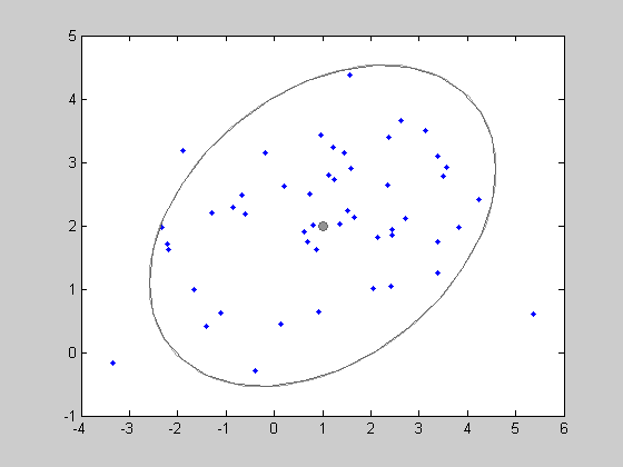
Random points generations . The object g can be used to generate a random samples from this distribution. Here, we generate 50 data points with the method RAND applied on the object g. This returns a 50x2 matrix x. We then plot the generated points. And isocontours of the density g can also be shown by the function show.
x = rand(g,50);
clf;
plot(x(:,1),x(:,2),'.');
show(g);
Giving the following figure:
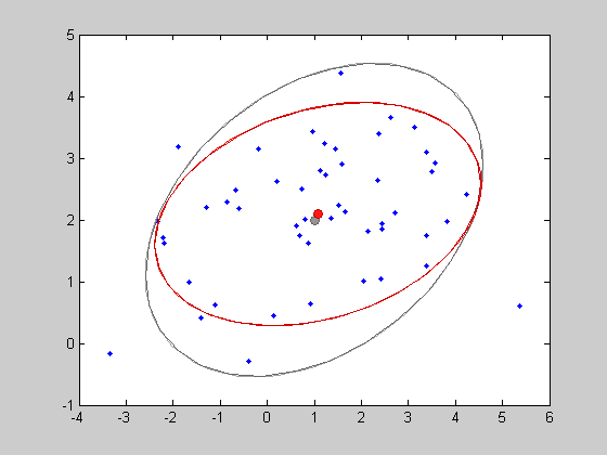
Parameters estimation . Now it is possible to find the Maximum Likelihood estimator of the mean and variance parameters. For gaussian distributions, the solution is closed form. Note that the ML estimator of the covariance is biased, but this bias is small (of order 1/n). The estimation is very simple: the method LEARN can be applied to any object of class DENSITY. Now we get the estimated model:
gest = learn(gaussdens,x)
gaussdens density:
m'  = [1.08 2.09]
var = [3.73 0.537
       0.537 1.01]
This estimated model can be plotted in red on the same picture.
show(gest,'color',[1 0 0])
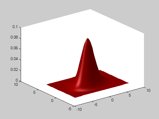
The function SHOW has various plotting possibilities. For example, one can prefer ploting the density values in the z axis instead of the isocontours.
clf;
show(gest,'color',[1 0 0],'mode','surf');
view(3)
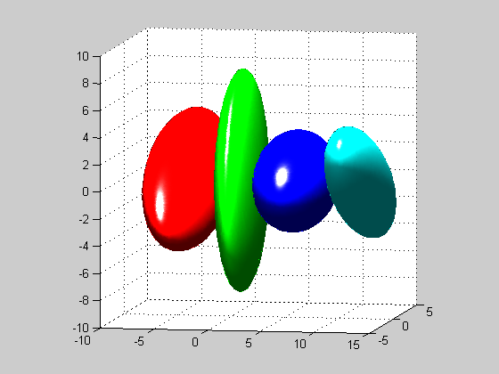
Constrained gaussian distributions . Often, in high dimensional settings, the full covariance matrices are not satisfiying, due to the large number of parameters needed to define the covariance matrix components. Therefore, other type of gaussian distributions are defined: - DIAGDENS: diagonal covariance matrix, - BALLDENS: spherical covariance matrix, - PCADENS: reduced-rank covariance matrix with noise in remaining directions. We define 3-dimensional distribution (so that PCADENS can be different from BALLDENS or GAUSSDENS), and then show the 80% isocontours thanks to the SHOW3 function that plots the 3-dimensional distributions.
d1 = gaussdens('m',[-4,0,0],'var',[2 .5 -.5;.5 4 2;-.5 2 4]);
d2 = diagdens('m',[1,0,0],'var',[.6 2 10]);
d3 = balldens('m',[6,0,0],'var',2);
d4 = pcadens('m',[12 0 0]','proj_mat',[0 1.5 -1.5]','off_std',1);

clf;
show3(d1,'color','r');
show3(d2,'color','g');
show3(d3,'color','b');
show3(d4,'color','c');

axis square %avoid afine deformations of the plot
grid on %show the grid
view(10,6) %set azimut and elevation for the 3D view
Creation . Mixture distributions are MIXTDENS objects, overloading DENSITY objects, but contains an array of other DENSITY objects for the clusters. For example, we create a mixture of 2 gaussian distributions with full covariance matrices. We first define 2 GAUSSDENS objects g1 and g2, and pass them to the MIXTDENS constructor in an cell array. The proportions of the cluster will be set respectively to 40% and 60%
%first gaussian distribution
g1 = gaussdens('m',[1;2],'var',[4 1;1 2]);

%second gaussian distribution
g2 = gaussdens('m',[3;-2],'var',[2 -2;-2 3]);

%and now, the mixture distribution
mxt = mixtdens({g1,g2},'prop',[.4 .6]);

%We can display informations about this distribution
mxt
mixtdens density object (2 clusters)
  cluster 1 (40%): gaussdens density:
    m'  = [1 2]
    var = [4 1
           1 2]
  cluster 2 (60%): gaussdens density:
    m'  = [3 -2]
    var = [2 -2
           -2 3]
This distribution can be used as previous ones, to generate random sample and to show the isocontours. One can notice that some specific features are added by the show function to the plot: the clusters are symbolized by ellipses.
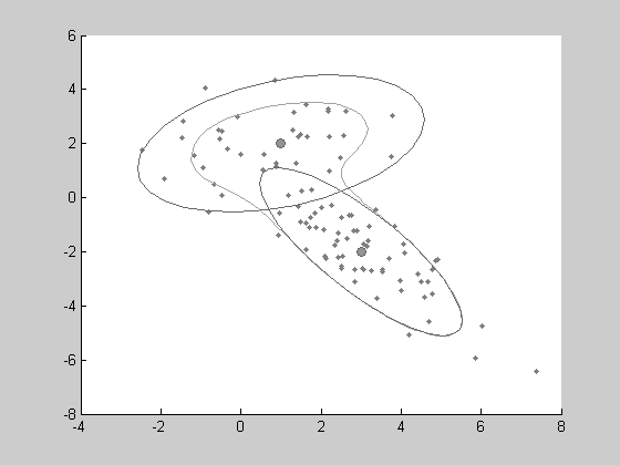
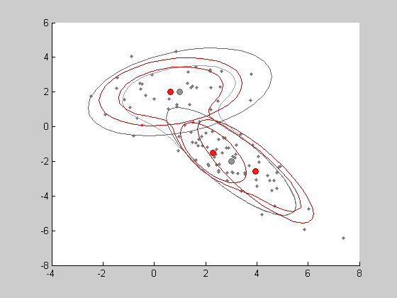
learning parameters by EM algorithm . As the previous distribution, the LEARN method is simply applied to an empty object containing a given number of clusters. Here, we will choose 3 clusters to see if the EM algorithm still find the 2 main generating clusters.
%estimation of a mixture model on the data matrix x

K=3 % number of clusters in the estimated model

%estimated model
mxtest = learn(mixtdens(gaussdens,K),x)

show(mxtest,'color',[1 0 0]) %plot the estimated distribution in red

%here are the estimated parameters
K =

     3

mixtdens density object (3 clusters)
  cluster 1 (33%): gaussdens density:
    m'  = [2.3 -1.51]
    var = [0.517 -0.459
           -0.459 0.939]
  cluster 2 (30.1%): gaussdens density:
    m'  = [3.94 -2.57]
    var = [1.59 -1.73
           -1.73 2.76]
  cluster 3 (36.8%): gaussdens density:
    m'  = [0.642 2.01]
    var = [2.42 0.422
           0.422 1.2]
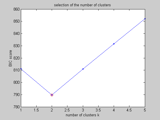
Model selection . If we do not know a priori the number of clusters, we can ask how many clusters are needed. One method to choose this number of clusters is to use the minimum value of the BIC criterion: BIC(t) = -2 * LL(t) + nu/2 log(n) where LL(t) is the maximum value of the likelihood, nu is the number of parameters and n the number of samples. This criterion can be easily computed by the methods LOGLIK and N_PARAMS, but a appropriate method BIC_SCORE already exists.
%to compare the models, we estimate the model with
% different numbers of clusters (from 1 to 5):

bics = zeros(1,5);
all_models = cell(1,5);

for k=1:5
   all_models{k} = learn(mixtdens(gaussdens,k),x);
   bics(k) = bic_score(all_models{k},x);
end
[bicmin,ind]=min(bics);

%now we can plot the computed bic values
%In the following figure, we shoul find the minimum value for k=2 %clusters

clf;
plot(bics,'.-');
xlabel('number of clusters k');
ylabel('BIC score')
title('selection of the number of clusters');
line(ind,bicmin,'Color','r','Marker','o');
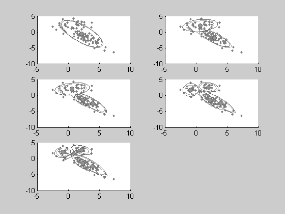
%All the estimated models can be plotted with only one function show %applied on the cell array of DENSITY objects

clf;
show(all_models,x);
Conclusion . We hope this tutorial showed helped you to anderstand how statlearn can help you to easily manage complex multidimensinal distribution. Many advanced features were not mentioned in this introduction, and we encourage you to see the help pages. For example, type 'doc unsupervised', or 'doc statlearn' for a complete presentation of the toolbox fonctions.